The main error propagation algorithm in iolite was first published by Paton et al. (2010). Its purpose is to estimate the additional uncertainty to be added to the internal uncertainty calculated by iolite and is most often used in U-Pb studies. We’ll focus on U-Pb for this Note but the algorithm is available for all data processing in iolite. Below we’ll cover how the algorithm works, and a new tool for examining the process. An alternative approach for calculating excess uncertainties, using iolite’s Database, will also be referred to below.

Why do we need to add additional uncertainty?

The default uncertainty reported by iolite is the spread of values within the selection for each channel. For example, the uncertainty for ‘Final 206Pb/U238’ is the uncertainty, for a selection, on the points in that channel for that selection. What Paton et al. discovered early on is that when we look at repeat measurements of a homogeneous material (e.g. secondary reference material) the spread in values is larger than what we’d expect given the uncertainties on each measurement. When I say “expect” here, I’m referring to the concept of a Mean Squared Weighted Deviation or “MSWD” which is more properly known as a Reduced Chi-Squared Statistic, but the term MSWD has been used in the geochronology community for decades and so that’s what we’ll use here. The basics of the MSWD is that is presents a single statistic ($\chi^{2}$) that we can use to examine our uncertainties relative to the dispersion of our measurements:

$$\chi^{2} = \frac{1}{\upsilon}\sum_{i}\frac{\left(O_{i} - C_{i}\right)^{2}}{\sigma_{i}^{2}}$$

where \(O_{i}\) is the \(i\)-th measurement, \(C_{i}\) is the computed value, \(\sigma_{i}^{2}\) is the variance of measurement \(i\) and \(\upsilon\) is the degrees of freedom. In geochronology, the MSWD rule(s) of thumb are:

• If the MSWD = 1: the uncertainties are consistent with the distribution of measured values

• If the MSWD < 1: the uncertainties are larger (on average) than the differences between the observed and calculated, and so may be “over-estimated” (i.e. the uncertainties are too large)

• If the MSWD > 1: the uncertainties are smaller (on average) than the differences between the observed and calculated, and so may be “under-estimated” (i.e. the uncertainties are too small).

This is based on the concept that our measurements for a homogeneous material should be scattered about the computed value by the same amount as the variance (i.e. the standard deviation squared).

In very simple terms, we can calculate the MSWD of our final U-Pb ratios (where the computed value is mean ratio) and if the MSWD is greater than 1, we know that there are potentially other sources of uncertainty not accounted for, and that we should add additional uncertainty until the MSWD is equal to one.

Calculating the Excess Uncertainty

In iolite we usually have our primary reference material (RM), which everything is normalised to, and secondary reference materials to check how well our process works. Paton et al. made the decision to keep the secondary reference materials out of the error propagation so that they could still be used for validation. This means that the algorithm uses the primary reference material to estimate the excess uncertainty. This can’t be done on the final ratios (e.g. Final 206Pb/238U) because at that point in the DRS the measured ratios have already been normalised to the accepted value, so they should all be equal the accepted value (± any smoothing in the spline). Instead, the downhole fractionation-corrected 206Pb/238U ratio is used as this is before normalisation to the accepted value but after baseline subtraction and downhole fractionation correction. We don’t use the mean of the measurements, as there is still sensitivity drift in these results. Instead, we calculate the difference between each measurement and a spline running through these measurements (this is the calculated value in our equation above). This difference is referred to as a “Jack-knifed” value.

Using our rule(s) of thumb above, if our uncertainties are correct, the average difference should be equal to the average variance of the measurements and our MSWD will equal one. However, typically for our reference material our spline will pass through each measurement (or close to it). Instead of having differences of close to zero, we take each primary reference material out of the pool of reference material measurements, and respline the remaining measurements. This new spline is then used to calculate the Jack-knifed value. We do this for all our primary reference material measurements, except the first and the last, because removing these and recalculating the spline give an unconfined spline for those measurements and we may get quite strange values for these two measurements. Our pool of measurements then is the primary reference material measurements, excluding the first and last measurement.

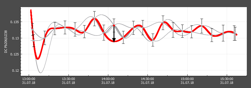
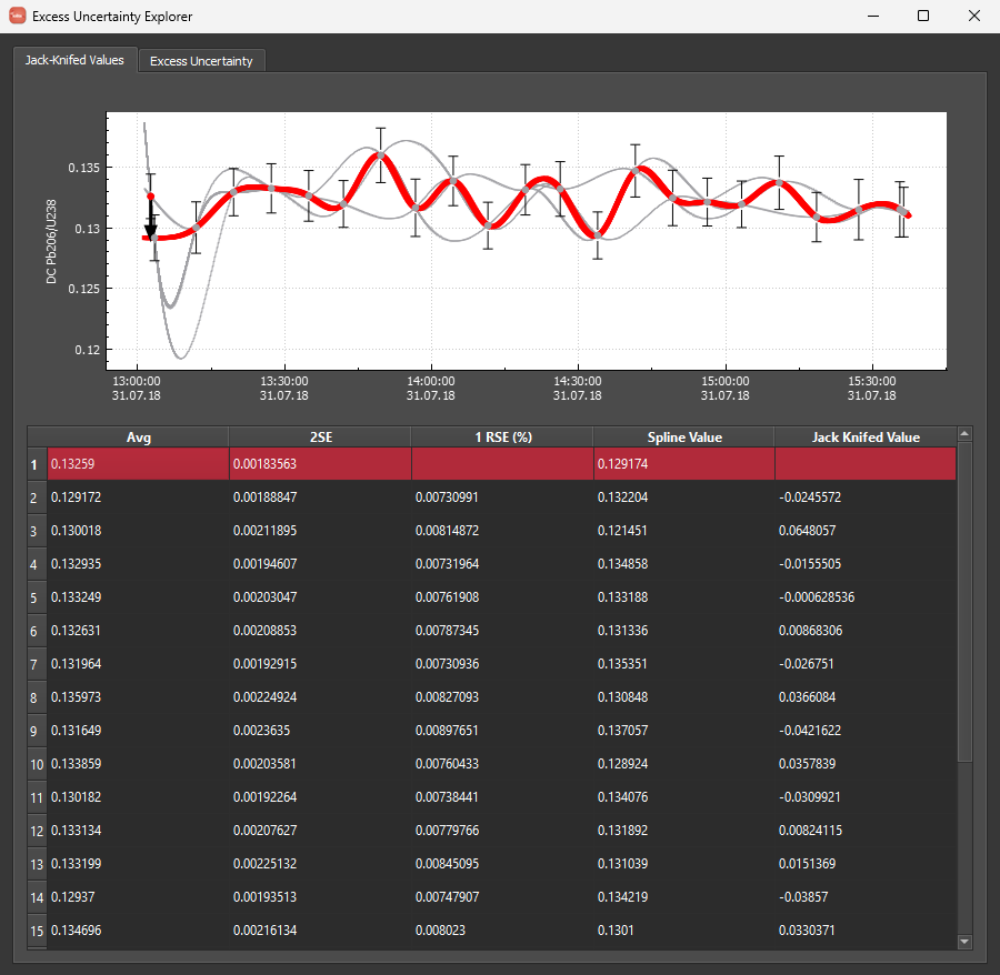
In the screenshot above, we can see an example Jack-knifed values calculation. A single RM measurement has been selected (red circle) from the pool of RM measurements (grey circles) and the spline calculated without this value is shown as a thick red spline. The other splines are those calculated where other RM measurements have been removed. The difference between the selected measurement and the spline (i.e. the Jack-knifed value) is shown as a thick black vector.

Where we have less than about 13 RM measurements, our MSWD is likely to be unreliable (too few measurements) and so iolite will not calculate the excess uncertainty if there are less than 15 primary RM measurements (15 measurements, minus the first and last, is 13 measurements for our MSWD calculation).

At this point we have a set of Jack-knifed values, and we can calculate the MSWD using these. The process of finding how much excess uncertainty to add involves adding a little extra uncertainty to the measurement uncertainties and recalculating the MSWD until we get an MSWD of roughly one. The additional uncertainty is calculated as a percentage of the measurement, and is added in quadrature. This way measurements with large uncertainties have a relatively smaller excess uncertainty added to them, and vice versa for measurements with smaller uncertainty. Because the excess is calculated as a percentage it can then be added in quadrature to other results including our final ratios. iolite keeps a record of the internal and excess + internal (propagated uncertainty) so that both can be plotted, examined and exported. The excess uncertainty (as %1RSD) for each output channel can be found in the channel’s properties, along with the channel the excess uncertainty was calculated from (in the Channel Browser).

A note about the spline type: sometimes it might appear that using a spline with no smoothing might be the best approach as it always passes through each RM measurement. However, between each measurement the spline can sometimes have steep positive and negative curves so that it can pass through each measurement (we’ll see an example of this below). If your sample is normalised to this potentially very rapidly changing curve, your normalisation value might be very different depending on how close it is the reference materials, and so it might have quite a large correction applied to it. Conversely, a very smoothed spline (e.g. a linear fit to all data is an example of a very smoothed spline) might have a consistent correction factor, but its lack of accuracy in modelling, for example, sensitivity changes will produce less accurate results. So we want to find some balance between the two. This is what the “Auto-smoothed” spline attempts to do, but depending on your results and experiment setup, it may not always produce what you want and so you should always check your splines.

The Excess Uncertainty Explorer

The Excess Uncertainty Explorer (EUE) is a user interface plugin for iolite v4. You can download it from iolite’s public GitHub repository (see this Note about downloading from GitHub). There are two files that need to be downloaded:

• ExcErrorExplorer.ui
• Excess Uncertainty Explorer.py

Both files need to be placed in the your iolite folder -> Plugins -> User interface. You can find the location of this folder in iolite’s Preferences, in the Paths section.

After placing the files in this folder, restart iolite if it is already running, and there should be an ‘Excess Uncertainty Explorer’ item in iolite’s Tools menu. Clicking on that will open the tool, but you should load a U-Pb experiment (.io4 session) where the processing has been completed before opening the tool.

In the example below, we’ll be using the DRO4 example dataset that was used for the U-Pb webinar. You can download this dataset and process it following the U-Pb webinar.

When you open the EUE, the window has two main tabs: Jack-knifed Values, and Excess Uncertainty. The Jack-knifed values tab shows the primary RM measurements for the downhole corrected 206Pb/238U (‘DCPb206/U238’) relative to the measurement time. Below that graph is a table showing each measurement. Selecting a measurement in the table will highlight it in the graph at the top. Highlighting a measurement shows that measurement as a red circle (the remaining will be grey circles), the spline that was calculated without that measurement (bold red spline) and the Jack-knifed value (a bold black vector). The table also shows these values for each measurement. This graph helps to show the effect of the spline type chosen. To see how it changes with different degrees of smoothing, close the EUE, change the spline type for the primary RM in the Time Series View, re-crunch the DRS and then reopen the EUE. No smoothing will create the very different splines shown in the example above. Change the spline type to maximum smoothing and reopen the tool to see the difference in Jack-knifed values.

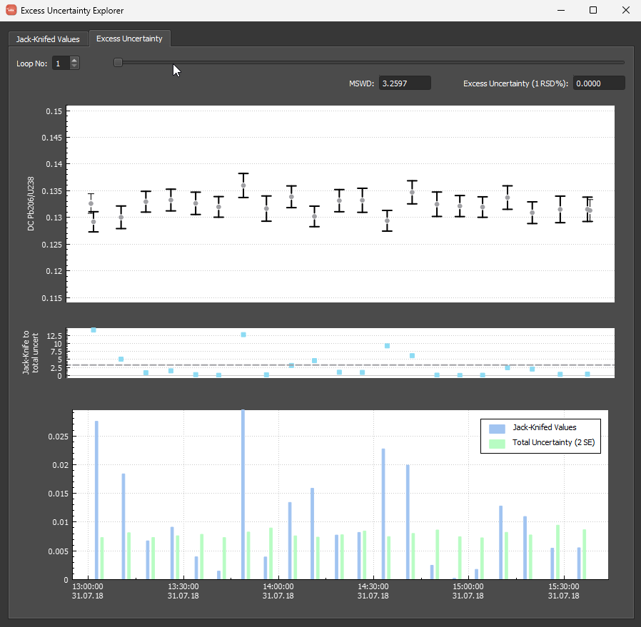
The second tab shows the Excess Uncertainty calculation (shown below). iolite calculates the excess uncertainty as an iterative loop, increasing the excess uncertainty until an MSWD of approximately one is reached. To visualise this process, at the top of this tab is a slider showing the loop number and the MSWD and excess uncertainty for this loop. You can advance the loop by dragging the slider to the right, or using the spin box on the far left (labelled ‘Loop No:'). For each iteration, the MSWD, excess uncertainty and graphs will update.

The upper plot shows each measurement with its internal uncertainty show as thin error bars. The propagated uncertainty (i.e. the internal + excess uncertainty) is also shown as thick error bars (initially the internal and propagated uncertainties will be the same). The bottom plot shows the Jack-knifed values (blue bars) and the propagated uncertainty for each measurement. Recall that an MSWD of one is where the average ratio between Jack-knifed value and uncertainty is approximately equal. The middle plot shows the ratio between the Jack-knifed value and the propagated uncertainty for each measurement. A dashed line in this plot shows the average ratio (i.e. the MSWD).

As the loop progresses, you’ll see the propagated uncertainty increase (the Jack-knifed values remain unchanged), and the average ratio between the Jack-knifed values and propagated uncertainty approach one. At the completion of the loop, you’ll be able to see the final MSWD and excess uncertainty (note that the algorithm doesn’t try to get an MSWD of exactly one as it has some degree of tolerance built in). This final excess uncertainty is the value used to calculate the propagated uncertainties for the output channels. Originally iolite only calculated the excess uncertainty using DC206Pb/238U, but now it calculates a unique excess uncertainty for 206Pb/238U, 207Pb/235U, 208Pb/232Th and 207Pb/206Pb. It is expected that these excess uncertainties will all be very similar, but slightly larger for 207Pb/235U, and quite a bit larger for 208Pb/232Th in zircon studies due to the decreased count rates of 207Pb, 208Pb and 232Th in most zircons.

We recommend changing your spline type and seeing what effect it has on the final excess uncertainty. In the DRO example dataset, changing from an auto-smoothed spline to an un-smoothed spline changes the excess uncertainty calculated from 0.0117% RSD to 0.0265% RSD, respectively. Although this is an exaggerated example, it helps to understand the effect spline type has on the final propagated uncertainties.

Summary and Alternative Approaches

We hope that this tool helps to explain how the Paton et al. approach works. We also note that there are other ways of determining excess uncertainty. In the Database webinar, we outlined an approach of using long-term secondary reference material results to calculate an excess uncertainty, and we feel this may be more accurate. However, the Paton et al. approach does not require a long-term dataset, can be calculated for an individual experiment, and retains the secondary reference materials as validation materials.

If you have any questions or suggestions about this approach, please feel free to discuss it on the forum.