One of iolite’s key capabilities is its ability to model processes occurring with a measurement session as time series. This is achieved via a series of interpolation methods, collectively referred to here as “splines” although they range from a simple mean of the observed data through to variably smoothed cubic splines. This Note outlines the interpolation methods available in iolite v4, along with an introduction to the mathematics that underpin the smoothed spline, with references to more detailed information.

Mean or median (“MeanMean” and “MeanMedian”)

This is a simple mean (or median) of the selection means within the group being interpolated. Note that the way the selection “mean” is calculated is set in iolite’s Preferences, in the Stats section. This can be a mean, median or geometric mean, with varying degrees of outlier rejection. We always recommend using the geometric mean for any data involving ratios.

Linear and Weighted Linear Fit

The interpolated values using this option are a linear fit, optionally taking into account the weight (uncertainty) of each selection. Selections with greater uncertainty will affect the less and vice versa.

Step Linear, Step Forward, Step Backward, Step Average and Nearest

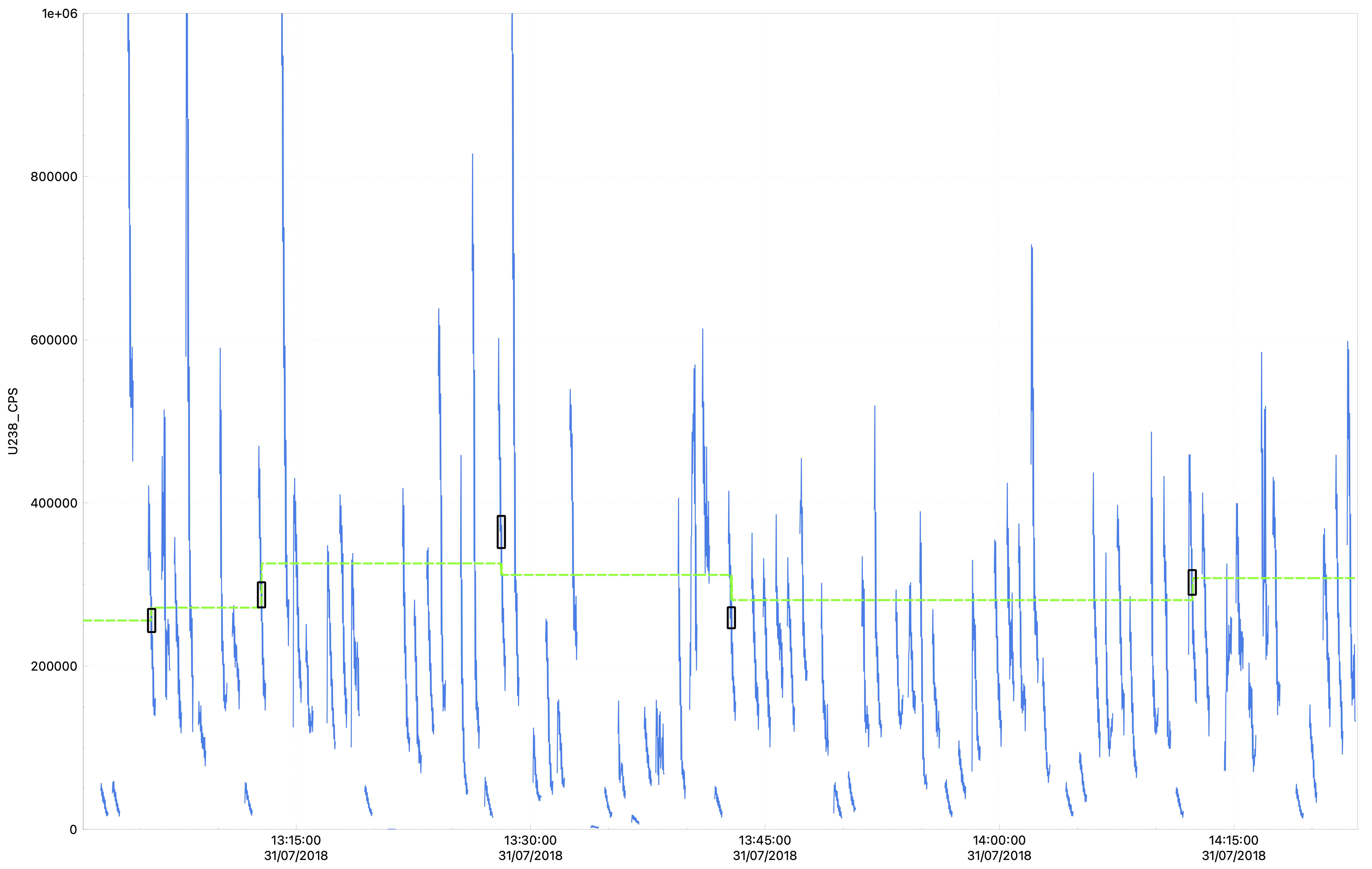
These methods create stepped interpolations that are flat between measurements (selections), or in the case of Step Linear some linear fit between the selections. The Step Forward option takes the mean (see note above about mean/median/geometric mean) value of a selection and remains constants until it reaches the start of the next selection. It then takes the mean value of that selection and remains constant until it reaches the next selection and so on. An example of a Step Forward interpolation is shown below.

The Step Backward interpolation is the same as the step foward option except that the value remains constant until it reaches the previous selection. This can be useful, for example, if your baseline measurement is more representative after an ablation, rather than before. In this example, the value of the baseline selection after the ablation will be used over the duration of the ablation.

The Step Average interpolator takes the average of the selection and the next and the value remains constant between the middle of the current selection and the middle of the next.

The Nearest interpolator takes the average value of the nearest selection and remains constant until another selection is closer in time.

The Step Linear interpolator fits a line between the mid point of a selection and the next selection.

Akima

The Akima interpolator uses an Akima spline to fit the data. The Akima spline is relatively stable in the presence of outliers.

Smoothed Splines

There are a range of smoothed spline options for fitting your data. These range from no smoothing, to maximum smoothing, with an autosmoothed option. To understand the smoothing parameter, it is useful to know that smoothed splines try to find a function $f(x)$ that minimises the following function:

$ \sum_{i=1}^n \left[ \frac{Y_i - f(x_i)}{w_i} \right]^2 + \lambda \int f^{\prime\prime}(x)^2 dx $

where f(x) is our interpolated function, $Y_i$ is the mean of selection $i$, $x_i$ is the time value of selection $i$, $w_i$ is the weighting of each measurement (the inverse variance of the selection), and $\lambda$ is the smoothing factor (greater than or equal to zero).

To gain some intuition about this minimised function, the first part that is being minimised ( $ \left[\frac{Y_i - f(x_i)}{w_i}\right]^2 $ ) is the difference between the interpolated values $ f(x_i) $ and the observed values $Y_i$, weighted by the uncertainty. By minimising this, we choose a function f(x) that most closely matches our observations.

The smoothing parameter $\lambda$ adds a penalty for increasing curvature. That’s the second part of the equation being minimised: $\lambda \int f^{\prime\prime}(x)^2 dx $. The integral of the second derivative is effectively the curvature of the function f(x), and lambda is how much penalty to apply for the curvature of the spline. For example, having a smoothing factor ($\lambda$) equal to 0, the function can fit the data exactly and the spline is free to “bend” in any way it needs to fit the data. Conversely, having large values of $\lambda$ mean that functions with higher curvature will be more penalised, and so as lambda gets larger, the fit will start to appear the same as a linear fit.

The auto-smooth option uses the mean square error (MSE) of the data points calculate an optimum value of lambda. We use the algorithm outlined in Hutchinson, 1986 which is available online, for free.

Extrapolation in iolite v4

Splines are typically evaluated between the first and last data point. But sometimes the first selection in our group is some amount of time after the start of our experiment, and similarly our last selection may be before the end of our experiment. To determine what values the spline should take before the first selection and after the last selection (i.e. extrapolation rather than interpolation) depends on the spline type.

For mean and median the values are the same before the first selection and after the last selection as the rest of the experiment. For the linear and weighted linear fits, the values before the first selection and after the last selection will match the values of the line fit to values within the selections.

For the Step functions, the spline before the first selection is equal to the average of the first selection and after the last selection is it equal to the average of the last selection.

For the spline functions (including the Akima spline interpolation method) the gradient and intercept of a line between the first/last selection and a point very close to that selection (e.g. 100 milliseconds after the midpoint of the selection) is calculated. The gradient and intercept is then used to create a line extending before or after the first or last selection, respectively. This has the effect of making the spline look linear beyond the first or last selections (rather than a curved cubic spline within the data points).

Click here to discuss.